Learning JEPA
How I-JEPA works, explained simply, and what happened when I tested it on CIFAR-100
Cover part of a photo, and you can still guess roughly what's behind your hand. You don't picture every pixel. You just know "that's probably more wing". JEPA teaches a network to do the same, without any labels.
The main architecture
I-JEPA is the version of JEPA for images. It has three networks that work together.
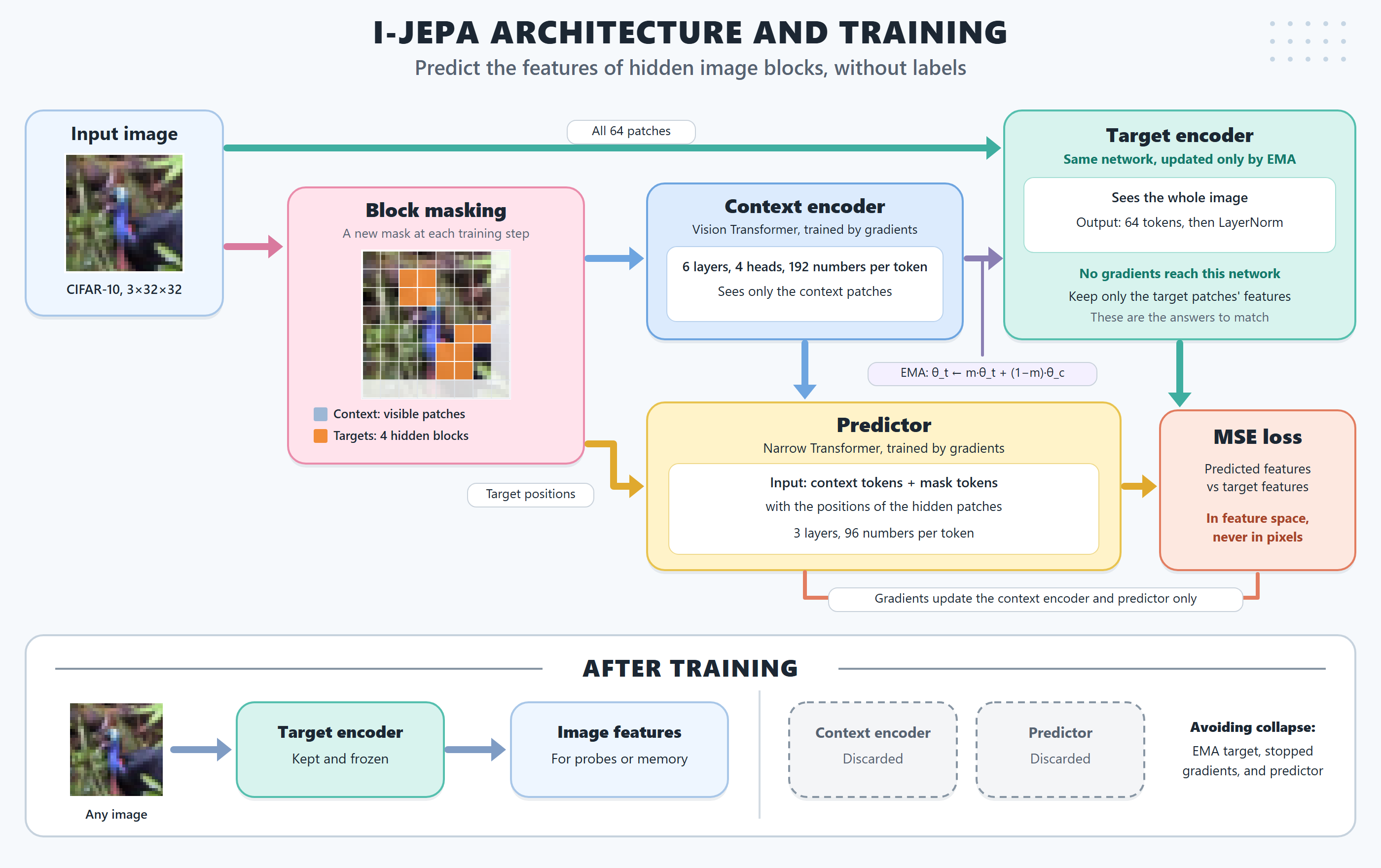
- Hide: choose some blocks of the image to hide.
- Look: the context encoder sees only the visible patches.
- Guess: the predictor guesses the description of the hidden patches.
- Check: the target encoder sees the whole image and gives the answer to compare with.
- Learn: the error trains the context encoder and predictor, and the target encoder slowly follows.
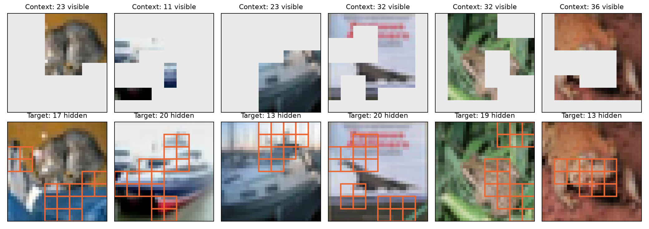
The three parts, one at a time
1. Context encoder: looks at what's visible
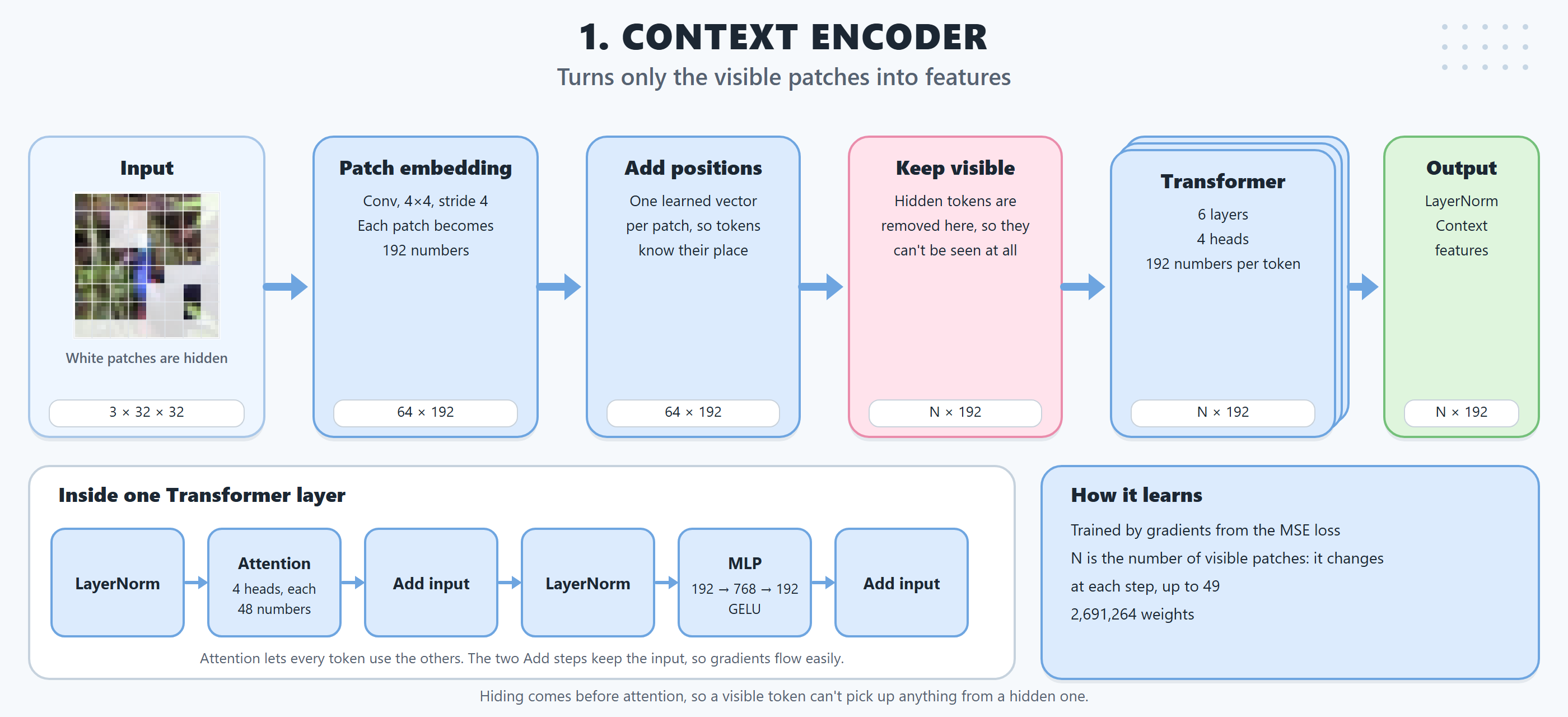
It cuts the image into patches, removes the hidden ones and describes the rest. Hidden patches are removed before attention, so it can't peek at them. It learns by gradients.
2. Target encoder: gives the answers
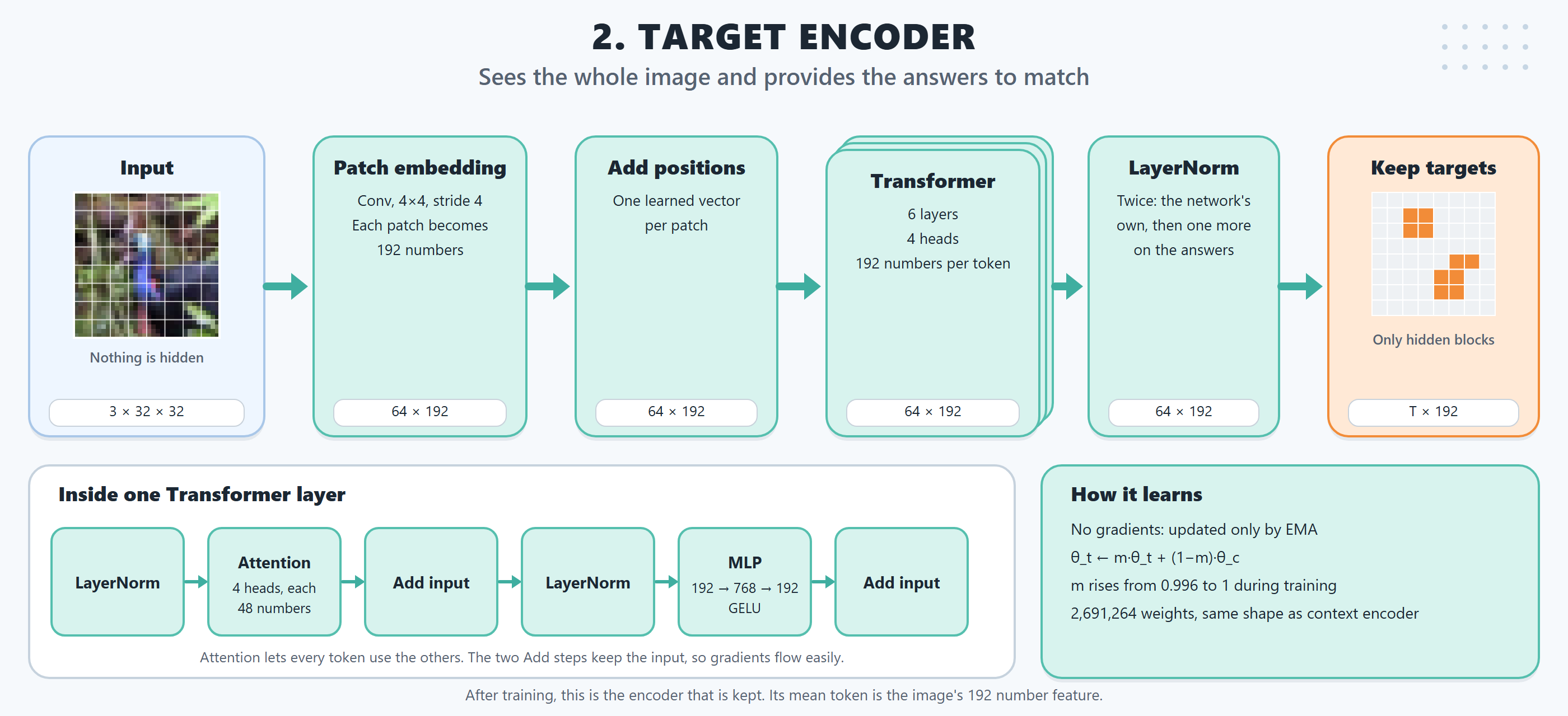
It has the same structure, but it isn't trained by gradients. After every step, it moves slightly towards the context encoder. This is called EMA, and nothing is copied across only at the end:
target weight = 0.996 × target weight + 0.004 × context weight
The 0.996 rises towards 1 during training, so the target changes more and more slowly. After training, this is the encoder that's kept.
3. Predictor: makes the guess
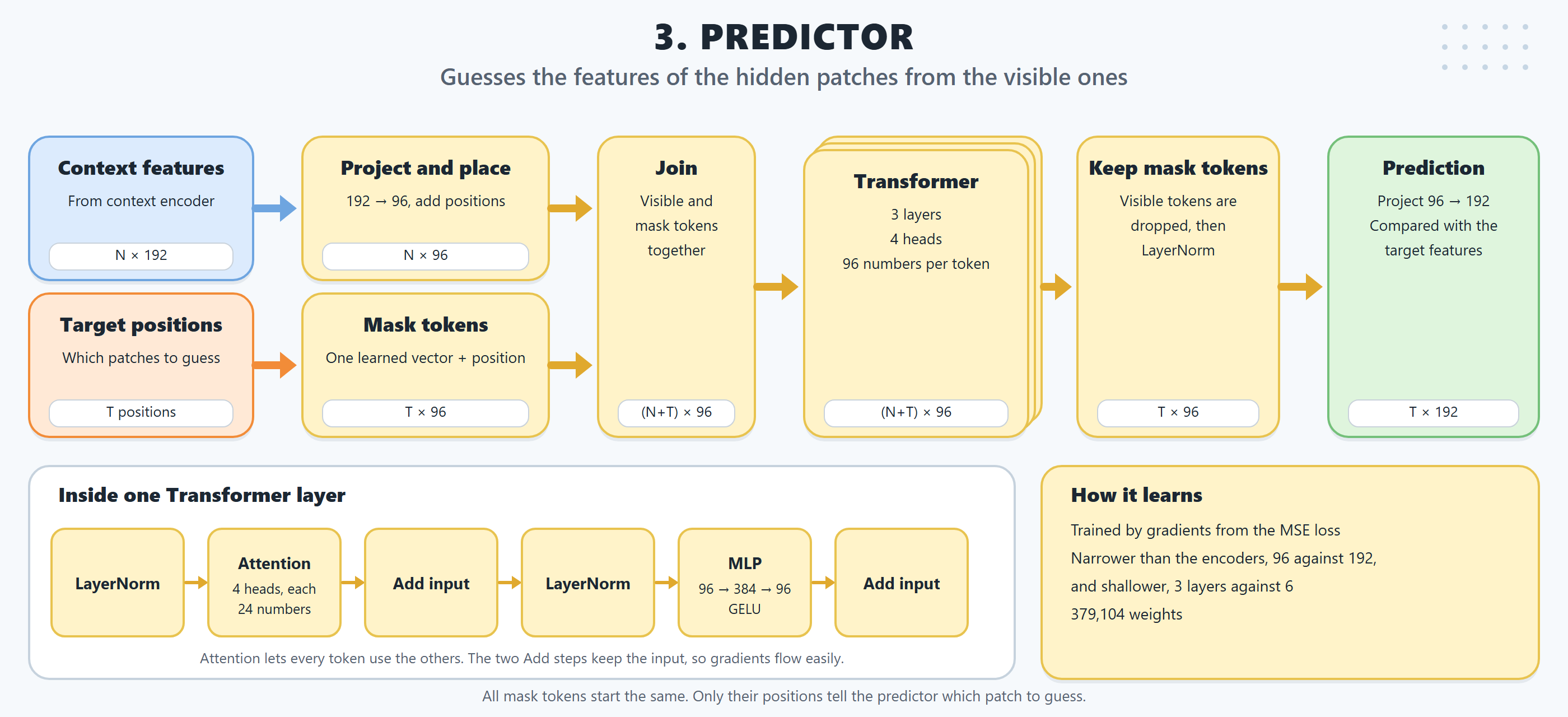
It's a smaller network. It receives the visible features, plus a "blank" mask token for each hidden patch with that patch's position. After training, it isn't needed for image features.
Inside the encoder: the Vision Transformer
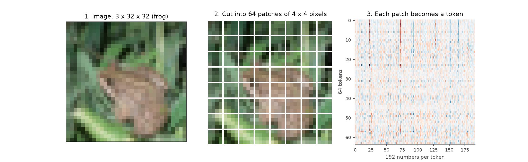
Both encoders are Vision Transformers (ViT). A ViT treats an image a bit like a sentence, with patches as its words. Our small one works like this:
| Step | What happens | Shape |
|---|---|---|
| 1. Image | A small colour photo | 3 × 32 × 32 |
| 2. Patches | Cut into small squares of 4 × 4 pixels | 64 patches |
| 3. Tokens | Each patch becomes a list of 192 numbers | 64 × 192 |
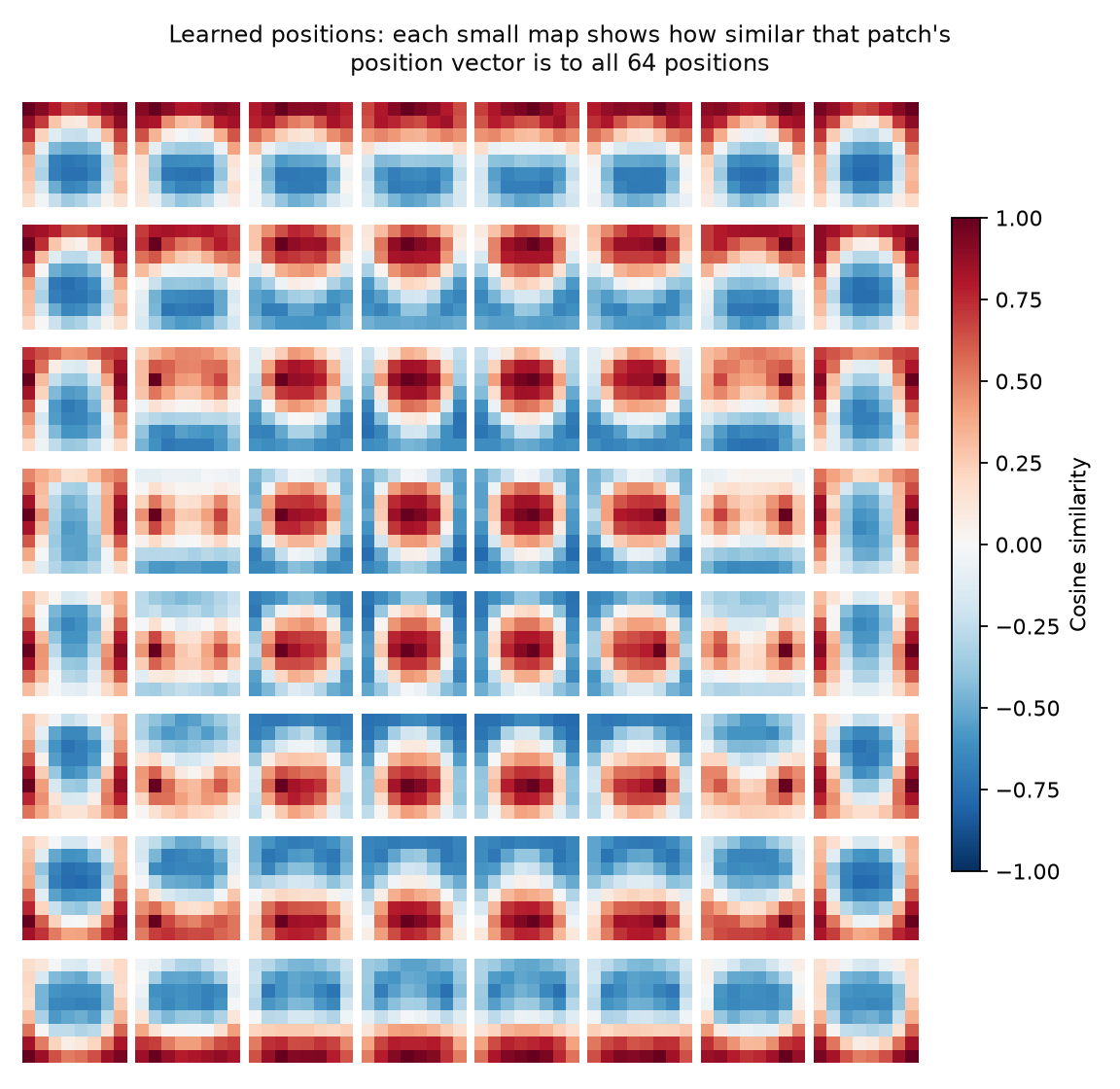
| 4. Positions | Add a learned vector saying where each patch was | 64 × 192 |
| 5. Transformer layers | 6 layers, each with attention and a small MLP | 64 × 192 |
| 6. Image feature | The average of the tokens | 192 numbers |
Attention, in plain words
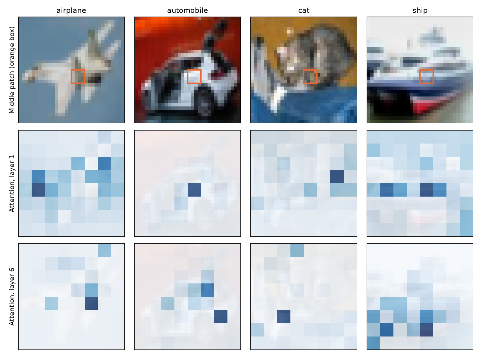
Attention lets every patch look at every other patch and borrow useful information. Each token makes three things:
| Part | Plain meaning |
|---|---|
| Query | "What am I looking for?" |
| Key | "What do I offer?" |
| Value | "Here's my information." |
Each query is compared with every key. Good matches get larger weights, and each token becomes a weighted mix of the values. This runs in 4 "heads" at once, so different heads can look for different things.
Why positions matter
Attention compares content, so it has no idea where a patch came from. I tested this with a supervised ViT, trained with labels, as a check on the encoder alone:
| CIFAR-10, 20 epochs, 3 seeds | Normal images | Patches shuffled |
|---|---|---|
| With positions | 81.05% ± 0.27 | 57.00% ± 0.58 |
| No positions | 73.90% ± 0.32 | 73.90% ± 0.32 |
Without positions, shuffling changes nothing at all: the network really can't see layout. This test used labels, so it isn't JEPA.
Show where attention looks
The experiment on CIFAR-100
Can a robot-style memory learn new classes using I-JEPA features? I replaced ResNet in CBCL and CBCL-PR, from Dr Ali Ayub's work, with I-JEPA. I call this side experiment Jepa-CBCL-PR.
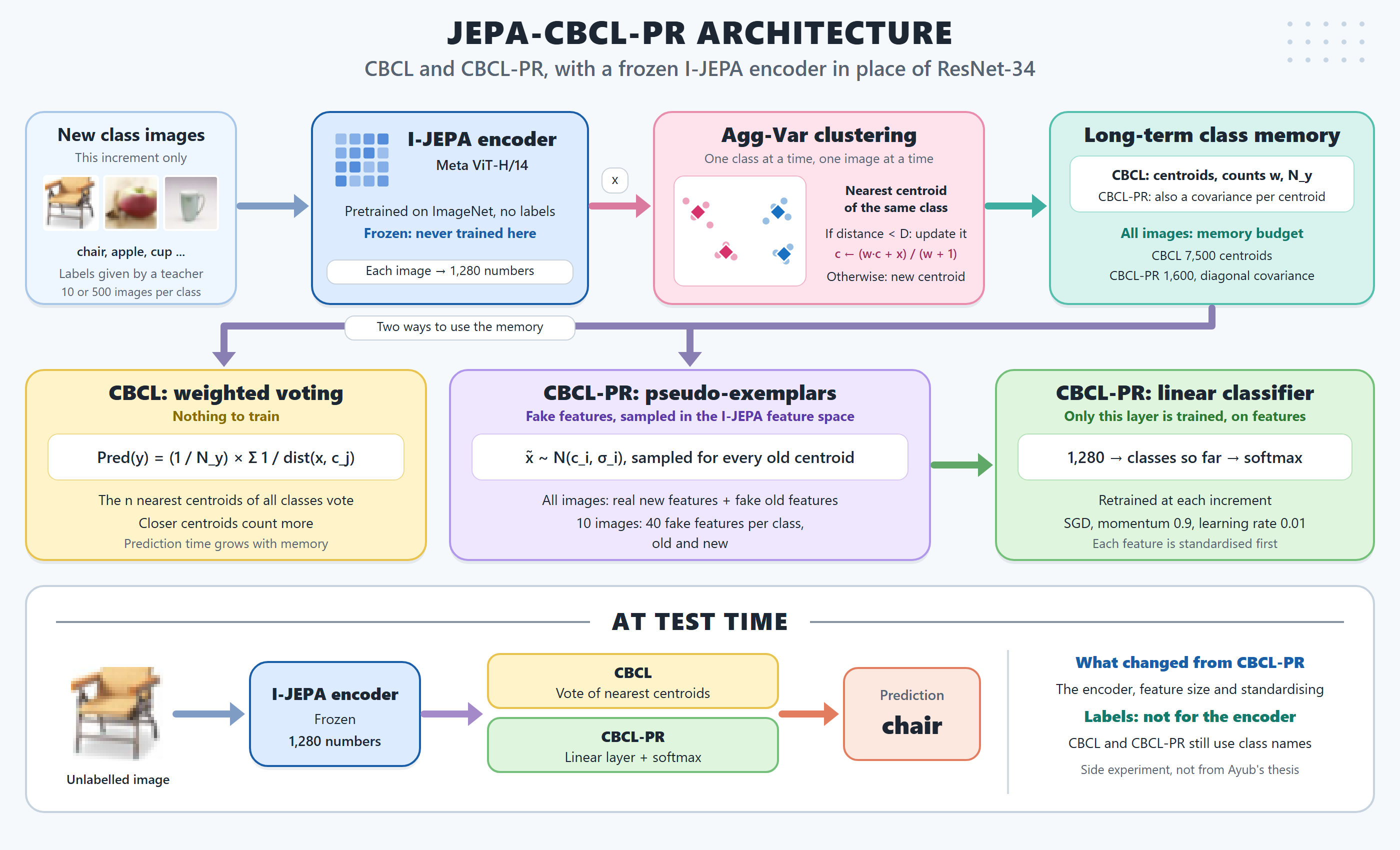
- Data: CIFAR-100, with 100 classes. Tested on all 10,000 test images.
- Teaching: 10 new classes at each of 10 steps, then a test on all classes so far.
- Images per class: 10, or all 500.
- With all images: memory is limited, to 7,500 centroids for CBCL and 1,600 for CBCL-PR, which uses diagonal covariance.
- Compared with: ResNet-34, our small I-JEPA and an untrained encoder.
- Reference: the same classifier trained on all the real features at once.
Time and epochs
How each encoder was trained
| Encoder | Trained on | Labels? | Epochs | Training time | Epochs on CIFAR-100 |
|---|---|---|---|---|---|
| Meta I-JEPA, ViT-H/14 | ImageNet-1K, by Meta | No | 300 | Not known to me | 0 |
| ResNet-34 | ImageNet, pretrained in torchvision | Yes | Not checked | Not known to me | 0 |
| Our small I-JEPA | 50,000 CIFAR-10 images, by me | No | 60 | About 26 minutes | 0 |
| Untrained small encoder | Nothing | — | 0 | — | 0 |
What ran for this test
On an RTX 4060 laptop GPU, measured from the run log.
| Step | Details | Time |
|---|---|---|
| Features from Meta's model | 60,000 images, enlarged to 224 × 224 | 21 min |
| Comparison, Meta I-JEPA | All methods and settings, 2 or 3 runs each | 21 min |
| Comparison, small I-JEPA | Same | 10 min |
| Comparison, untrained encoder | Same | 9 min |
| Comparison, ResNet-34 | Same, using features saved earlier | 9 min |
| All comparisons | After the features were ready | 49 min |
Epochs inside the test
| Part | What it trains | Epochs |
|---|---|---|
| CBCL | Nothing. It builds centroids and votes | 0 |
| CBCL-PR | A linear classifier, retrained at each step: SGD, learning rate 0.01, momentum 0.9, batch 64 | 25 to 70, rising by 5 per step |
| Reference | The same classifier, all at once | 70 |
Results
Show these values as a table
Final accuracy on all 100 classes
Percent, mean ± standard deviation. Chance is 1%. There are 3 runs with 10 images, 2 runs with all images, and 1 reference run with all images.
What this shows
- A strong encoder matters most. With CBCL-PR, Meta's I-JEPA beat ResNet-34 by about 12 points in both settings: 64.06% against 51.66%, and 74.23% against 62.59%.
- That isn't proof that JEPA beats CNNs. Meta's model has about 30 times the weights of ResNet-34, and I didn't test a large supervised model.
- Fake features have a cost. With all images and limited memory, CBCL-PR scored 7 to 11 points below learning everything at once, for our three trained or pretrained encoders.
- Our small I-JEPA fell well behind on new classes, at 26.67%. It still beat the untrained encoder's 10.53%, so it learned something that transfers.
- Memory can be small. Meta's 1,019 centroids need about 10 MB, against about 256 MB for all its real features, calculated from their sizes.
Limits
- Not an equal contest: the encoders differ hugely in size.
- Tiny images: CIFAR-100 images are enlarged from 32×32 to 224×224 for the larger encoders, which adds no real detail.
- "New" is partial: some CIFAR-100 objects resemble things in ImageNet or CIFAR-10.
- Few runs: 2 or 3 per version, with one teaching schedule.
- Not comparable with the thesis: features are standardised here, and this isn't part of my CBCL reproduction.
- What the predictor really knows: on our small model, tests showed it uses the visible patches, but they didn't show that it predicts a hidden patch's own content. The dashboard has that test, under Learn → Lesson 5.
Credit
- I-JEPA: Assran et al., "Self-supervised learning from images with a joint-embedding predictive architecture", CVPR 2023. Paper.
- Pretrained model: facebook/ijepa_vith14_1k, licensed CC BY-NC 4.0, for non-commercial use.
- CBCL and CBCL-PR: Ayub and Wagner, CVPR Workshops 2020 and IEEE TCDS 2023. This experiment isn't affiliated with the authors.